To add conditional formatting to cells, you select those cells and create a so-called formatting rule for them. Formatting rules always consist of two parts:
▪a condition
▪... and the formatting to be applied when this condition is met
Example: "If the cell content is greater than 1000, display it in red color."
Application example
To define (and apply) a formatting rule like this, proceed as follows:
| 1. | Navigate to the desired cell. Of course, you can also select multiple cells to apply conditional formatting to them together. |
| 2. | On the ribbon tab Home | group Format | Conditional formatting |
| Tip: For quick use of common formatting rules, you can also bypass the dialog box by applying certain options directly from the dropdown menu of the command Conditional formatting (see "Tip: Applying formatting rules directly from the dropdown menu" below). |
| 3. | In the dialog box, first select for Type, which type of condition should be used. |
| In our example, you would select Format only cells that contain. (For detailed information on each type of condition, see Types of conditional formatting). |
| 4. | Next, specify the desired condition. |
| In our example, this would be the condition "cell value is larger than 1000". Accordingly, select the options Cell value and greater than. In the edit control at the right, type in the value 1000. |
| 5. | In the last step, click on the Format button and specify the formatting options to be applied whenever the condition is met. |
| In our example, switch to the Font tab, set the font color to Red and confirm with OK. |
| 6. | All necessary settings are now completed. Click on OK to confirm and create the new rule. |
The new formatting rule is now created – and at the same time applied to the selected cells. This has the following effect:
▪If the cell content is smaller than or equal to 1000, the cell will be displayed in its original format.
▪If the cell content is greater than 1000, the cell will be displayed in the conditional format, that is, in red color.
Note: You can create as many formatting rules for a cell (or cell range) as you like. For example, you can add a second rule that formats the cell in boldface if it contains a value below zero etc. etc.
Tip: Applying formatting rules directly from the dropdown menu
If you choose the ribbon command Home | group Format | Conditional formatting ![]() , you can apply certain frequently used formatting rules directly from the dropdown menu.
, you can apply certain frequently used formatting rules directly from the dropdown menu.
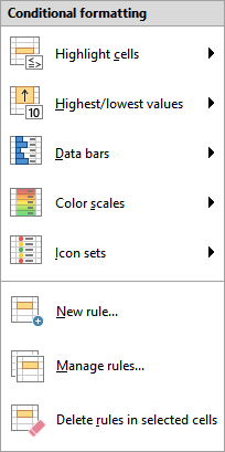
The following types of formatting rules are available in the upper area of the dropdown menu:
▪Highlight cells: see description in the next section "Types of conditional formatting", paragraph Format only cells that contain ...
▪Highest/lowest values: see description in next section "Types of conditional formatting", paragraph Format only upper or lower values
▪Data bars, Color scales, Icon sets: see description in next section "Types of conditional formatting", paragraph Format all cells based on their values
In the submenus, click on More rules to open the dialog box with even more differentiable setting options, if required.