With the ribbon command View | group Windows | Freeze cells ![]() you can fix the first rows and/or columns of a table on the screen. As a result, that they no longer move when scrolling through the worksheet, but permanently stay in place.
you can fix the first rows and/or columns of a table on the screen. As a result, that they no longer move when scrolling through the worksheet, but permanently stay in place.
This is particularly useful if you have put headings into rows or columns of a worksheet, and want these headers to stay visible all the time.
Activating freezing
To freeze rows or columns, you can use the following options:
▪Only freeze the top row: Use the small arrow of the icon Freeze cells, and select the entry Freeze top row. It does not matter which cell you have selected before.
▪Only freeze the first column: Use the small arrow of the icon Freeze cells, and select the entry Freeze first column. It does not matter which cell you have selected before.
▪Freeze the top row and first column: Choose the two commands of above one after the other to combine freezing the top row and the first column.
▪Freeze any number of lines: If you want to freeze the first rows (without freezing columns), proceed as follows:
| In the row header on the far left, select the row directly below the rows you want to fix. Then click directly on the icon Freeze cells. |
| Alternatively: Use the icon's small arrow and select the entry Freeze at current position. |
▪Freeze any number of columns: If you want to freeze the first columns (without freeze rows), proceed as follows:
| In the column header at the top, select the column to the right of the columns that you want to fix. Then click directly on the icon Freeze cells. |
| Alternatively: Use the icon's small arrow and select the entry Freeze at current position. |
▪Freeze any number of rows and columns: If you want to freeze several first rows and columns, place the cell frame in the cell right below the area you want to freeze. Then click directly on the icon Freeze cells.
| Alternatively: Use the icon's small arrow and select the entry Freeze at current position. |
The rows and/or columns are now frozen. They remain in their original location when you scroll through the worksheet.
Tip: You can also use the icon ![]() in the bottom-right corner of the document window to freeze rows or columns. Simply click this icon and then drag it to the desired location.
in the bottom-right corner of the document window to freeze rows or columns. Simply click this icon and then drag it to the desired location.
Disabling freezing
If you have fixed rows or columns, the icon Freeze cells ![]() is shaded darker to indicate that freezing is enabled. To disable it, click again directly on the icon itself – the rows/columns are no longer fixed.
is shaded darker to indicate that freezing is enabled. To disable it, click again directly on the icon itself – the rows/columns are no longer fixed.
Alternatively: Use the icon's small arrow and select the entry Unfreeze cells.
Tip: A single mouse click on the icon ![]() in the bottom-right corner of the document window will also disable freezing.
in the bottom-right corner of the document window will also disable freezing.
An example
Assume you have the following worksheet:
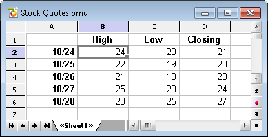
Note that both the columns and the rows are labeled. To freeze the labels, proceed as follows:
▪The column labels (High, Low, etc.) are in the first row of the table.
| To freeze them, select the second row by clicking its row header (the button left of the row, labeled with "2"). |
| Then select the ribbon command View | Freeze cells. |
▪The row labels (10/24, 10/25, etc.) are in the first column of the worksheet.
| To freeze them, select the second column (column B) by clicking on its column header (the button above the column, labeled with "B"). |
| Then select the ribbon command View | Freeze cells. |
▪To freeze both rows and columns, click cell B2 and select the ribbon command View | Freeze cells.
Tip: Since it is the top row and first column in this example, you might as well use the commands Freeze top row and Freeze first column by clicking the on the arrow of the icon Freeze cells.
If you want to unfreeze, click on the icon Freeze cells again.