If you have named cell ranges using the ribbon command Formula | group Named ranges | Edit names ![]() , you can perform various operations much more efficiently.
, you can perform various operations much more efficiently.
In practice, you use named ranges as follows:
Quickly selecting a named range
In the top-left corner of the worksheet window, you can see a dropdown list that displays the address of the currently selected cell.
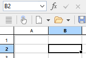
When you open this dropdown list, it will display a list of all named ranges. Clicking on one of these names will select the corresponding cell range.
Using names in formulas
In formulas, range names can be used instead of the cell addresses they represent. This saves time, but also makes formulas easier.
An example:
You have entered sales figures for January in cells A2 to A10. You have also assigned the name "January" to this range of cells.
To sum up the sales, you simply type:
=SUM(January)
This method is also considerably more understandable than the default naming convention of =SUM(A2:A10).
Of course you can now also name the sales for February, March etc. accordingly.
Tip: In the dialog box of the ribbon command Formula | Function ![]() there is also an entry called "Named ranges" in the Category list. If you select this category, all named ranges are listed in the Function list so that you can easily insert them into formulas.
there is also an entry called "Named ranges" in the Category list. If you select this category, all named ranges are listed in the Function list so that you can easily insert them into formulas.