PlanMaker lets you enter arrays (also known as matrices) in spreadsheets and perform calculations with them. An array A is a rectangular number scheme in the following form:
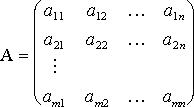
The entries a11 to amn are called the elements of the array. They are divided into m rows and n columns. This is why it is called an m x n array.
Entering arrays into corresponding cell ranges
To enter an array in PlanMaker, simply distribute the array's rows and columns over the worksheet's rows and columns.
For example, the following array ...

... has to be entered as follows:
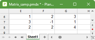
As you can see, each (rectangular) cell range can also be considered an array – and vice versa. Thus, for arithmetic functions that expect an array as an argument, you can always specify a cell range that contains the elements of the array.
Entering array formulas
PlanMaker provides array functions with which you can perform calculations with arrays – for example, find the inverse of an array. A formula containing an array function is called an array formula.
In contrast to "ordinary" formulas, array formulas only return an entire array of values rather than a single value. For this reason, such array formulas have to be entered in a different manner. Let's take a look at an example of this:
You want to determine the inverse of the 3x3 matrix shown above. To do so, proceed as follows:
| 1. | Select a cell range for the resulting array |
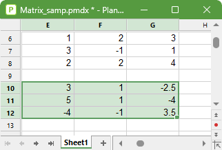
| Before entering an array formula, you have to select the cell range where the resulting array should be placed. The inverse of an array always has exactly as many rows and columns as the initial array. Thus, you have to select a range of 3x3 cells – for example, cells E10:G12. |
| 2. | Enter the array formula |
| Now enter the desired array formula. In our example, this would be the formula =MINVERSE(E6:G8). |
| 3. | Ctrl+Shift+Enter |
Important: To complete the formula, press the key combination Ctrl+Shift+Enter key rather than the Enter key.
The cells E10:G12 now contain the resulting array, i.e., the inverse of the array in E6:G8:
Notes:
▪If you have selected a cell range larger than the resulting array, the error value #N/A ("not available") will be displayed in the superfluous cells. Important: If the selected cell range is too small, parts of the array will not be displayed.
▪To edit an existing array formula: Select all cells of the resulting array, edit the formula and press Ctrl+Shift+Enter key. If you just press the Enter key instead, PlanMaker will issue a warning and ask you if you want to overwrite the array.
▪Tip: To select all cells covered by an array formula, click on one of these cells and then press Ctrl+7.
Note for users of Android/iOS:
Use the commands Insert array formula ![]() and Select array formula instead of the shortcuts Ctrl+Shift+Enter key and Ctrl+7. As the two commands are not displayed by default in PlanMaker, you must first add them to your user interface:
and Select array formula instead of the shortcuts Ctrl+Shift+Enter key and Ctrl+7. As the two commands are not displayed by default in PlanMaker, you must first add them to your user interface:
| 1. | Open the dialog box "Customize user interface" by choosing the command Tools > Customize via the hamburger menu |
| 2. | In the dialog box, enter the search term "array" in the quick search. The two commands are then shown in the list on the left. Add the commands to the list on the right as described in the section Customizing toolbar icons . |
Entering arrays with constants
If desired, arrays can be entered as constants instead of cell references. For this purpose, enclose the array within curly braces { }. Separate columns via commas and rows via semicolons.
For the array already used as an example above...
... you could also enter the following in PlanMaker:
={1,2,3;3,-1,1;2,2,4}
Explanation of the above notation
| 1. | First, the values of the upper row are entered after the curly bracket, with the values separated by a column separator: ={1,2,3 |
| Note: |
| The format of the column separator depends on your system's country settings. If, for example, Germany is set, use periods ={1.2.3 and if US is set, use commas ={1,2,3 |
| For languages like Spanish, for example, a backslash can also be used for the column separator in Microsoft Excel: ={1\2\3 This is not possible in PlanMaker. |
| 2. | You then have to enter a semicolon, which completes the row as a row separator : ={1,2,3; |
| Note: The semicolon as a row separator is the same for all country settings. |
| 3. | Then enter the middle row 3,-1,1 and complete it with the row separator: ={1,2,3;3,-1,1; |
| 4. | Finally, enter the last row 2,2,4 for the array formula: ={1,2,3;3,-1,1;2,2,4} |
Notes:
▪The notation described above is only permitted for fixed values; formulas and cell references are not allowed.
▪Of course, you can also enter vectors in the above notation. For a row vector such as a = (1, 2, 3), enter {1.2.3}; for a corresponding column vector, enter {1;2;3}.