That's enough theory for now! Let's now perform our first calculation.
First, we enter the price of the computer; under that, the price of the monitor; and under that, the price of the printer.
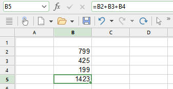
Thus, navigate to cell B2 and type the value 799 there. The value will appear both in the selected cell and in the Edit toolbar above the worksheet.
Note: When entering numbers, do not make the mistake of typing the letter "O" or "o" instead of the number "0". PlanMaker makes a clear distinction between letters and numbers. The letter "O" is not a number for the program. PlanMaker would accept the input but interpret it as text, and thus could not perform calculations with it.
Then press the Enter key↵ to complete your input. The cell frame automatically moves down one row to cell B3. Type the value 425 here and the value 199 in the row below.
Tip: If you entered an incorrect value and have already pressed the Enter key↵, you can still correct your mistake. Use the arrow keys to move the cell frame to the cell with the error, and enter the correct value. Then press the Enter key again, and the old cell content will be overwritten by the new input. You can also edit the content of already filled cells by pressing the F2 key.
Entering formulas
Let's enter our first formula.
In order to calculate the total cost of our computer equipment, we have to add up the unit prices that we just typed. This is very easy:
Go to cell B5 and type an equal sign = at first. The equal sign shows PlanMaker that you would like to start entering a formula in this cell.
Then enter the formula. For this purpose, you use the cell addresses as "variables". Enter the following:
=B2+B3+B4
Note: Cell addresses are not case-sensitive, i.e., you can enter them in either uppercase or lowercase.
When you press the Enter key↵, you will immediately see the result of your first formula in the cell:
Let's see what happens if you change the numbers in the cells. For example, navigate to the cell that contains 425 and enter 259 or some other value instead. As soon as you press the Enter key↵ again after replacing the cell content, the result of the calculation will be updated immediately.
Regardless of what cells B2, B3 and B4 contain, PlanMaker will always add them up. If you get a quote for a computer system in which only the price of the printer has changed, for example, you only need to change that particular value, and the new total price will be displayed in cell B5.
The "SUM" function
The above example is one method of adding up several numbers. Although the method is adequate for a few numbers, it is clearly too cumbersome for adding 50 numbers - that would be a very long formula! Fortunately, there are alternative methods: the computational functions of PlanMaker.
In order to find out more about them, make cell B5 the current cell; it contains the formula you entered previously.
First, delete the old formula by pressing the Del key on the keyboard or by simply overwriting the existing cell content. Then enter the following formula:
=SUM(B2:B4)
After pressing the Enter key↵, you will see the result in the cell: the sum of the cells B2 to B4.
PlanMaker has a whole range of computational functions – and one of them is SUM. As its name suggests, the SUM function calculates the sum of the relevant values. The expression in parentheses after the function name tells PlanMaker where to start and stop summing.
You have directed PlanMaker to start adding in cell B2 and stop in cell B4. In this case, only the number in B3 is in between, but the SUM function would also work with a larger range, such as B2:B123.
The notation Start cell:End cell also works across rows and columns. If, for example, you enter B2 as the start cell and C4 as the end cell, these two coordinates in the worksheet form the corners of a rectangle. The formula =SUM(B2:C4) would thus sum all numbers included within this rectangle.
Variety of formulas
To get an idea of the multitude of computational functions available in PlanMaker, you can now choose the command Function.
You will find the command on the ribbon tab Formula | Function ![]() or as Insert function with an identical icon in the Edit toolbar. Even faster: Simply press F7.
or as Insert function with an identical icon in the Edit toolbar. Even faster: Simply press F7.
The program will now display a dialog box with a list of all functions that PlanMaker supports.
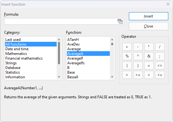
Tip: You can open a help page for each arithmetic function. Click on the desired function in the above dialog box, and then press the F1key.
Let's try another function. We'll calculate the average value of our three numbers in the worksheet:
To do so, exit the dialog box and delete the contents of B5 again.
Then choose the command Function (Insert function) ![]() . Select the "All functions" category in the list on the left side of the subsequent dialog box. Then scroll down through the list on the right to the "Average" function. Double-click on the "Average" function.
. Select the "All functions" category in the list on the left side of the subsequent dialog box. Then scroll down through the list on the right to the "Average" function. Double-click on the "Average" function.
In the input field Formula of the dialog box, PlanMaker has now automatically inserted the Average() row. To complete the formula, enter B2:B4 again between the parentheses.
Alternatively, you can simply select the desired cell range directly in the worksheet by left-clicking on cell B2 and then dragging the mouse down to cell B4. If the dialog box is covering the cells that you want to select, simply drag it out of the way while holding down the mouse button.
The completed formula should look as follows:
=Average(B2:B4)
If you click on Insert, this formula will be transferred to cell B5 and calculated immediately.
You have now learned about two of the more than 400 computational functions of PlanMaker. For a comprehensive list of all functions, see Functions from A to Z.