You can use the Group function to display data even more clearly. For example, group the dates in your pivot table report by years, quarters or months to make time periods more meaningful.
You will find the command for this as the Group... button at the bottom of the pivot table sidebar.
An example:
You have created a pivot table from the familiar sample data (see Creating a new pivot table).
Then, proceed as follows:
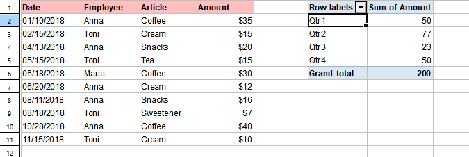
| 1. | In the pivot table sidebar, drag the Date field to the Row labels area and the Amount field to the Values area. |
| 2. | In the pivot table report, select a cell with a date value. |
Note: Only one cell may be selected at a time.
| 3. | Click on the Group... button in the pivot table sidebar. |
| 4. | In the dialog box that now appears, select the entry Quarters from the list, for example. |
| 5. | In the dialog box, confirm with Group. |
The pivot table report then shows the following result: The amounts are summed quarterly.
The "Group..." function in detail:
Depending on the contents of a selected cell, you group date values, numeric values or text. Multiple groupings in the same pivot table are possible, both for Row labels and Column labels.
After you have selected a cell in the pivot table and clicked on the Group... button, one of the following dialog boxes opens, each with different options:
▪The dialog box Group by dates appears if the selected cell contains date values:
| With the Auto options enabled, the date values are preset to a range with the first and last date of all records and are thus grouped for this period. If you want to customize the time period, disable the Auto checkbox in front of the input fields Starting at or Ending at and enter the desired values there. |
| In the list below, select the time unit (Months, Quarters, etc.) by which you want to group. Click with the mouse on the corresponding entry from the list, which is then highlighted in blue and is thus selected. To deselect, click again on the entry highlighted in blue. Tip: You can also select multiple time units by just clicking on another entry. For example, it may make sense to select Days as well as Quarters. The days are then shown in the pivot table for the relevant quarter. |
| Once you have made your choice, press Group in the dialog box. |
| Note: The input field Number of days is only available if you have selected Days as the only unit of time in the list above. This option causes the pivot table to display the specified number of days as a time interval from...to and is especially useful for displaying the results of calendar weeks. To do so, enter the number 7 and disable the two Automatic options above. For Starting at, select the Monday before the oldest date of your source data (this would be 01/08/2018 in the example above) and, for Ending at, the Sunday after the most recent date (1/18/2018 in the example). |
▪The dialog box Group by numbers appears if the selected cell contains numeric values:
| With the Auto check boxes enabled, the numeric values are preset to a range with the smallest and largest numeric value of all records. The numeric values in this range are thus grouped. If you want to customize the range, disable the Auto checkbox in front of the input fields Starting at or Ending at and enter the desired values there. |
| You use the option By below to determine at which intervals the numeric values are to be grouped. You thus receive a summarization to value classes. If, for example, you enter 0 for Starting at, 40 for Ending at, and 10 for By, you will obtain the classes 0-19, 10-19, 20-29, 30-39 by which your records will be grouped. |
| Finally, press Group in the dialog box. |
▪The dialog box Group text appears if the selected cell contains text:
| In the Labels list on the left, select the items that you want to group by clicking on them with the mouse. The entry now appears highlighted in blue. To deselect an item, simply click on it again. |
| Important: In the input field Group name, first type a name. It is only then that you can then use the New group button to create a grouping for the selected items. You can then add more groups in the same way by selecting items from the left list again and entering a group name (ensure that you confirm with New group). |
| In the Groups list on the right, you will see the result of the created group(s): The group name at the top and the items it contains below. |
| If you want to rename a group, select the corresponding group in the Groups list on the right. Important: In the Group name field, type the new name first, and then click on the Rename group button. |
| Use the buttons |
| Finally, click on OK in the dialog box. |
Ungrouping
To reset grouped data, select a cell of the grouping in your pivot table report. Click on the Ungroup button in the pivot table sidebar. Only the grouping of the field to which the selected cell belongs is reset.
Alternatively, you can click on the Group... button to open the dialog box again and click on the Ungroup button there.
Only for cells with text: If you have created several groups for a field with text, you can remove a single group via the dialog box by selecting a group in the dropdown list on the right and using the Ungroup button. The Ungroup all button, on the other hand, ungroups all groupings for this field (corresponds to the Ungroup button in the sidebar).