The previous section described how to apply conditional formatting to cells. In the dialog box that appears, you can choose between the following types of formatting rules:
Format all cells based on their values
This type of conditional formatting does not actually use a condition at all. In fact, it reformats all of the previously selected cells – based on the values they contain.
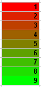
If, for example, you choose a 2-color scale from red to green, the lowest value will be highlighted in red and the highest value in green. The colors for the values in-between will be calculated automatically. The result will be a color gradient as follows:
There are several different subtypes for this type of formatting rule. They can be selected via the option Format style. This contains the following entries:
▪2-color scale
| This is described in the example above. |
▪3-color scale
| This is the same as the 2-color scale, but it also lets you set the color for the midpoint. |
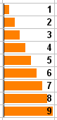
▪Data bars
| Here, bars that correspond to the relative size of the value are displayed in the background of the cells – similar to a bar chart: |
 |
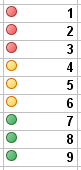
▪Icon sets
| This displays an icon in each cell, indicating the size of the respective value – for example, a red signal light for the lower third of the values, a yellow one for the middle third and a green light for the upper third: |
 |
Format only cells that contain ...
This type of rule reformats only those cells within the current selection that meet the specified condition.
Proceed as follows: First, specify the desired condition, using the controls and input fields in the dialog box.
Then, click on the Format button and specify the formatting options to be applied for all cells that meet the condition.
An example can be found in the previous section – where we created a formatting rule "If the cell content is greater than 1000, display the cell in red".
Format only upper or lower values
This type of rule reformats only those cells that contain the highest or lowest values within the current selection.
First, specify which values to reformat – for example, the top 3 values or the top 10% of the values.
Then click on the Format button and specify the formatting options to be applied to the corresponding cells.
Format values above or below average
This type of rule reformats only those cells that contain values above or below the average of the current selection.
First, specify which values to reformat – for example, all values above the average.
Then click on the Format button and specify the formatting options to be applied to the corresponding cells.
Format unique or duplicate values
This type of rule reformats all unique values (or duplicate values) within the currently selected cells.
First, specify which values to reformat:
▪all unique values (values that occur only once)
▪or all duplicate values (values that occur at least twice)
Then click on the Format button and specify the formatting options to be applied to the corresponding cells.
Use a formula to determine which cells to format
Here, only those cells are reformatted for which the specified formula returns TRUE.
To do so, enter the desired formula in the dialog box. Note that only formulas that return a logical value (thus, TRUE or FALSE) are permitted. See also notes below.
Then click on the Format button and specify the formatting options to be applied to the corresponding cells.
Some notes:
▪Creating suitable formulas
| You can use any kind of formula for the condition. You only have to ensure that the result of the formula is a logical value (thus, TRUE or FALSE). |
| Examples: |
| If you enter the formula "SUM($A$1:$C$3) > 42", the conditional formatting will be applied if the sum of the cell range A1:C3 is greater than 42. |
| If you enter the formula "ISEVEN(ROW())", the conditional formatting will be applied if the current cell is located in a row with an even row number. |
▪Using absolute and relative cell addresses
| Note that the formula can also use relative cell references in addition to absolute cell references (as in the above example). These are treated as follows: |
| An absolute cell reference – for example, $A$1 – always refers to cell A1. |
| On the other hand, a relative cell reference – for example, A1 – refers to the cell in the upper left corner of the selection. That means: |
| If you apply conditional formatting to an individual cell, A1 refers to the relevant cell. |
| If you previously selected a cell range, A1 refers to the cell in the upper left corner of the selection, A2 to the cell below it, etc. |