Use the command AutoFilter to filter the rows of a cell range:
When you select a cell range and choose the command Data | group Filter | AutoFilter, from now on, an arrow will appear on top of each column in this cell range. Clicking on one of these arrows opens a menu where you can easily choose between the values contained in the corresponding column – and other predefined filter conditions.
Note 1: The AutoFilter can only be inserted once per worksheet; two separate filters cannot be inserted on one worksheet. Otherwise, you cancel the previously applied filter by selecting the AutoFilter command again. If you have created Tables in worksheets, they have their own AutoFilters - even on the same worksheet.
Note 2: Newly added or updated values are not automatically sorted by the previously set filter conditions. To integrate changed data into existing AutoFilter, use the command Reapply filter.
Proceed as follows to apply the AutoFilter:
| 1. | Select the desired range of cells. Important: The first row of this range must contain headings for the data below. |
| 2. | Choose the command Data | group Filter | AutoFilter |
The AutoFilter function is now enabled. Note the downward arrows in the first row of every column in the selected range.
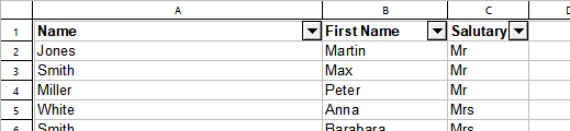
Clicking on one of these arrows ![]() will open a menu listing the contents of the current column, as well as some other options. By default, all values in the list are selected, meaning that currently no filtering is taking place.
will open a menu listing the contents of the current column, as well as some other options. By default, all values in the list are selected, meaning that currently no filtering is taking place.
To filter the data in the cell range, use this menu as follows:
▪Sort ascending ![]() : Sorts the filter results of the applied AutoFilter range in ascending order.
: Sorts the filter results of the applied AutoFilter range in ascending order.
▪Sort descending: ![]() : Sorts the filter results of the applied AutoFilter range in descending order.
: Sorts the filter results of the applied AutoFilter range in descending order.
▪More filters (contextual): Text filters, Number filters and Date filters open a submenu with additional filters (see below).
▪(All): This menu entry is a useful placeholder: It allows you to add/remove all values the column contains with just one click.
| A check mark is displayed to the left of this entry to indicate that currently all cell contents are contained in the filter. |
| When you click on the entry (All) now, all cell contents are removed from the filter (and the check mark disappears). When you click it again, all cell contents will be added to the filter again (and the check mark reappears). |
| If not all cell contents are included in the filter, but at least one cell content, a gray area is displayed instead of the check mark. |
▪(Blank): If you have empty cell contents in your column, you can use this selection to show/hide all empty rows.
▪List of the cell contents: The most important part: This part of the menu lists all cell contents that the column contains. You can add/remove a value to the filter by clicking on it. A check mark is displayed to the left of all entries that are currently contained in the filter.
Note: For the last 3 described options (All), (Blank) and List of cell contents please always be aware: To confirm your selection, you have to press OK.
Example
For example, to filter a cell range in a way that it shows only rows that contain the name "Smith" in a column with the heading "Name", proceed as follows:
Select the cell range (including the column headers) and use the ribbon command Data | group Filter | AutoFilter to activate the AutoFilter.
An arrow ![]() now appears next to each column header. Click on the arrow for the column "Name" to open the AutoFilter menu for this column.
now appears next to each column header. Click on the arrow for the column "Name" to open the AutoFilter menu for this column.
First, click on the (All) entry in this menu in order to remove all cell contents from the filter. Then, choose the menu entry "Smith" and press OK. You have now created a filter condition "Name equals Smith" using the AutoFilter function. PlanMaker will hide all rows that do not match the condition.
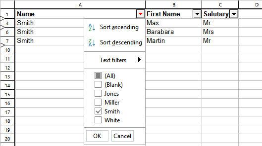
Filter result after the name "Smith" has been selected in the list of cell contents at the bottom of the AutoFilter
If, in addition, you would also like to have all rows with the name "Miller" listed, simply choose the menu entry "Miller" as well. To remove the Millers again, click on the "Miller" entry once more to deselect it. Press OK to confirm in each case.
If necessary, apply additional filter conditions in the other columns as well (e.g., "Mrs" for all female matches of a given name) to further narrow down the results.
As you can see, the entries in the AutoFilter menu can be combined in any possible way. Just click on an entry to add it to the filter – or remove it.
More filters: Text filters, Number filters, Date filters
Depending on the format category of the filtered columns, PlanMaker automatically sets more filter options for Text filter, Number filter or Date filter in the AutoFilter menu. The Text filter is offered for text-only values and the Date filter for date-only values. If the formats are mixed, the Number filter is applied.
Use the offered filter to obtain specialized filter conditions, for example:
Text filters:
▪Equals... Display only rows with exact matches.
▪Does not equal... Rows with exact matches are hidden.
▪Greater than... Display rows with values that are alphabetically behind the entered filter value.
▪Greater than or equal to... See above, but including the entered value.
▪Less than... Display rows with values that are alphabetically before the entered filter value.
▪Less than or equal to... See above, but including the entered value.
▪Starts with... Display only rows with specific word beginnings.
▪Doesn't start with... Rows with specific word beginnings are hidden.
▪Ends with... Display only rows with specific word endings.
▪Doesn't end with... Rows with specific word endings are hidden.
▪Contains... Display only rows that contain specific strings as part of the text.
▪Doesn't contain... Rows that contain specific strings as part of the text are hidden.
Number filters:
▪Greater than... Works like the operator > . Display rows with values that are greater than the filter value entered.
▪Greater than or equal to... Works like the operator ≥ . Display rows with values that are greater than or equal to the filter value entered.
▪Less than... Works like the operator < . Display rows with values that are smaller than the filter value entered.
▪Less than or equal to... Works like the operator ≤ . Display rows with values that are smaller than or equal to the filter value entered.
▪Between... Display values of the rows which are defined in a number range.
▪Not between... Hide values of the rows which are defined in a number range.
▪Top 10... Display only rows where the value in this column is amongst e.g. the 10 highest (or lowest) values. You can customize this selection when the Top 10... dialog box has opened: In the field on the left, choose between Top or Bottom values. In the middle field, you can set the number of top/bottom values. In the right-hand field, you can choose between absolute values (Items) and relative values (Percent).
| An example: |
| If you want to get 50% of the lowest values from 60 values given, then set the following: |
| Left field: Bottom Middle field: 50 Right field: Percent |
▪Only empty: Display only rows where the value in this column is empty.
▪Non-empty: Display only rows where the value in this column is not empty.
▪Above average: Display only rows where the value in this column is larger than the average value (of this column).
▪Below average: Display only rows where the value in this column is smaller than the average value (of this column).
Date filters:
▪Equals... Display only rows with exact date matches.
▪Does not equal... Rows with exact date matches are hidden.
▪Before... Display only rows in which the date values are earlier than the entered date value.
▪Before or equal... See above, but including the entered value.
▪After... Display only rows in which the date values are later than the entered date value.
▪After or equal... See above, but including the entered value.
▪Between... Display rows where the date values are within a defined date range.
▪Not between... Hide rows where the date values are within a defined date range.
▪Day, Week, Month, Quarter, Year: Here you can make further selections to quickly narrow down the desired date ranges.
| Note: If you have applied the AutoFilter to date values, you will notice in the dropdown list of the AutoFilter that the single days have already been sorted at year and month level. Click on the plus sign in front of the year/month level to expand it and view the associated single values. If you have now expanded the date "tree" and, for example, selected only single day values from a certain date level, in front of the associated date level (month/year) a gray area appears instead of a check mark. Only if all available values of a date level are selected, also a check mark for this level appears. If no value of a date level is selected, you will see a white area in front of it. This allows you to see at a glance whether all, none or single values of a date level have been selected. |
In addition, there are the following options for each of the offered filter methods Text filters, Number filters or Date filters:
▪Custom filter: Open a dialog box where you can define individual filter conditions.
▪Delete filter: This option is only available if criteria have been set via the Text filter, Number filter or Date filter selection. Press Delete filter to remove only the criteria applied through these filters.
Making all filtered rows visible again
If you want all rows hidden by AutoFilter to become visible again, choose the ribbon command Data | group filter | Show all.
If values in the cell range set by AutoFilter have changed, you can use the ribbon command Data | group Filter | Reapply filter to update the selection you have already defined.
For example, you have specified that all rows with the name "Smith" should not be displayed and further entries with this name were added afterwards. With the command Reapply filter you can filter out such subsequently created entries again and you don't have to define the terms of the filter again from the beginning.
Of course, this function is especially helpful for dynamic formula and date values.
Deactivating the AutoFilter
To completely disable the AutoFilter function, choose the ribbon command Data | group Filter | AutoFilter once again. The downward arrows displayed at the top of the cell range disappear, and all filtered rows will become visible again.