Now, let's return to our first sample worksheet. Although it has proved to be an accurate calculation here, it is not very attractive in terms of design. At the same time, PlanMaker has extremely powerful options for visually preparing worksheets.
Let's try some of them out:
Adding a headline
What is missing from our worksheet is a headline. So let's simply enter a text in a cell above the numbers and increase the font size to make it stand out.
Click on cell B1 to make it the active cell. Then, for example, type the following text:
My first worksheet↵
Changing character formatting
Next, let's choose a different font for the heading – and make it a lot bigger.
For this purpose, first move the cell frame back to the cell B1 again. Then expand the font list on the ribbon tab Home | group Character by clicking the small arrow to the right of the font name.
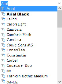
PlanMaker now displays a list of all fonts installed on your computer. Select the Tahoma font (or any other font you like).
Then open the font size list ![]() to the right (or below) of the font list and select size 24 point.
to the right (or below) of the font list and select size 24 point.
If desired, you can also set the font color ![]() , in the same command group you will also find three buttons labeled B, I and U for toggling bold, italics and underlining.
, in the same command group you will also find three buttons labeled B, I and U for toggling bold, italics and underlining.
Changing number formatting
When it comes to formatting numbers, PlanMaker not only allows you to change the character format of numbers (font, font size, etc.), but you can also modify their number format.
Let's try this out: To display the values in the cells B2 through B5 with a currency symbol, proceed as follows:
First, select the cells B2 to B5. To do so, click on the cell B2 and then – with the mouse button still held down – move the mouse cursor to the cell B5.
Android/iOS: If you are using these versions, please note that selecting text there works slightly differently. For more information, see Selecting cells and cell content.
When the desired cells are selected, click on the ribbon tab Home in the command group Number on the group arrow![]() in the bottom right corner. The program opens a dialog box with numerous options. We are only interested in the tab named Number format: On this tab, simply choose the entry "Currency" from the list and confirm with OK.
in the bottom right corner. The program opens a dialog box with numerous options. We are only interested in the tab named Number format: On this tab, simply choose the entry "Currency" from the list and confirm with OK.
Result: A currency symbol is now displayed with values in the selected cells. Also, the values are displayed with two digits after the decimal point.
There are many more number format options at your disposal. For example, you can make values display as percentages, change their number of decimal places, etc. Important: Applying a different number format to a value only changes its display – not the value itself.
You have now met a tiny part of PlanMaker's options for improving the visual display of worksheets. Many more are waiting to be discovered by you. For more information on this, see Formatting worksheets.