As mentioned in the introduction of the section Consolidating data, the command Data consolidation allows you to consolidate data from one or more cell ranges, for example, in order to calculate their total sums.
In the simplest case, data is consolidated by its position. This works as follows:
You have entered the data into e.g. three "source ranges". They should be identical in size and structure. In all three of them, each piece of data should have the same (relative) position.
When you let PlanMaker consolidate these cell ranges, it begins with calculating the sum of the first cell (top left) in the first range, second range and third range. The result appears as the first cell in the "target range". Then, the same is done with all other cells in each of the cell ranges.
Example
The daily revenues of two fruit shops are to be consolidated by means of a sum function, divided according to fruit varieties.
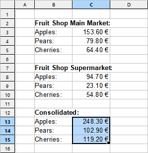
For this purpose, the revenues of the two shops were entered into a table. In the figure, this data is shown in the cell areas C3:C5 and C8:C10.
Then the command Data consolidation was executed and these two areas were added as source ranges. The target range was set to C13:C15 (selected in the figure) and consolidation was started.
Result: In the target range, the sums of the daily revenues appear (again per fruit variety, just as in the source ranges).
Performing a consolidation by position
To consolidate data by position, proceed as follows:
| 1. | Enter the data to evaluate into one or more cell ranges of exactly the same size and structure. The order of the individual pieces of data must be identical in each range. |
| The cell ranges can be located in just one worksheet altogether or be spread over multiple worksheets or even multiple files. |
| 2. | Choose the ribbon command Data | group Analyze | Data consolidation  . . |
| 3. | Click into the edit field below Source ranges. There, enter the address of the first cell range containing the data to evaluate. (See also notes below.) |
| Tip: Alternatively, with the dialog box still open, simply click into the table and select the cell range with your mouse. |
| 4. | Click on the Add button. |
| 5. | To add additional source ranges, repeat the steps 3. through 4. |
| 6. | At Target range, enter the address of the cell range where you want the results of the consolidation to be inserted. |
| Tip: It is sufficient to specify just the address of the cell in the top left corner of the target range. PlanMaker will then determine its size automatically. |
| Tip: You can simply click on the desired cell in the table to transfer its address into the dialog box. |
| 7. | At Function, choose the arithmetic function to be used for the consolidation. |
| 9. | Click on Apply to start the consolidation. |
The data from the source ranges is now consolidated using the chosen arithmetic function. The result is inserted in the target range.
Note: The result of a consolidation is inserted into the table as fixed numbers. These numbers will not be updated when you modify the values in any of the source ranges.
Accordingly, this command's main purpose is to evaluate the current state of data, not regarding any changes made to them later (useful e.g. for monthly reports). See also Editing and updating consolidations.
Notes on specifying the source ranges
In the dialog box described above, the Source ranges control can be used to add a source range in the following ways:
▪Source range from the current worksheet
| To add a cell range that is located in the current worksheet to the source ranges, simply enter its address or name. |
| Tip: Alternatively, with the dialog box still open, you can click into the table and select the cell range with your mouse. |
▪Source range from a different worksheet
| To add a cell range that is located in a different worksheet, enter its address preceded with the other worksheet's name and an exclamation mark. |
| Tip: You can also select the cell range directly in the table with your mouse. Make sure that you have clicked on the desired worksheet in the worksheet register first. |
▪Source range from a different document
| To add a cell range that is located in a different document, enter its address the same way that external references are entered (see External cell references). |
| Example: 'C:\My Folder\[My Workbook.pmdx]Sheet3'!D2:G5 |
| Tip: You don't have to enter the first part of the address (folder and file name) manually. When you click on the Browse button in the dialog box, a file dialog appears, allowing you to choose the desired file. |
Don't forget to click on the Add button every time you have completed entering the address of a source range.