You can also import data records from other PlanMaker files or Microsoft Excel files to create a pivot table. To do so, proceed as follows:
| 1. | Choose the ribbon command Insert | group Tables | Pivot table  . . |
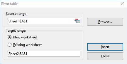
| The following dialog box opens: |
| In the file browser, locate the file with your source data and confirm with Open. |
| The input field below Source range displays the file path with the file name and a proposed worksheet with a cell area. Here you have to adjust the desired cell range precisely. PlanMaker does not automatically extend the cell range to corresponding data records when importing from external files. |
| Example: Your source data is in the file Pivot.pmdx in the worksheet Sheet1, and the cell range of your source data records is from A1 to D11. |
| The syntax in the input field is then: 'filepath\[Pivot.pmdx]Sheet1'!$A$1:$D$11 |
Tip: If you have previously named the range of source data in your external file (see Naming cell ranges), you can avoid entering the cell range exactly. A further advantage of this procedure is that you have to adjust the named range only when making changes to the data records. Choose the name of the named range in the input field using the following syntax: 'filepath\[filename]'!name
| 3. | Target range: Here you can decide where the pivot table should be created: |
| New worksheet: The pivot table will be created in a new worksheet that is automatically generated by PlanMaker. You can adjust the proposed target in the lower input field. |
| Existing worksheet: The pivot table will be created in an existing worksheet. This can be the worksheet containing the source data or another existing worksheet. Please make sure that you first select the radio button Existing worksheet and then click with the mouse on a cell in a free area in the desired worksheet. Or type the target range into the lower input field. |
| 4. | Confirm with the Insert button to create the pivot table. |
You should now see a (still blank) Pivot table report in the worksheet and the so-called Pivot table field list or just Field list on the right in the sidebar. It is the dialog and the central control of the pivot table. By selecting the elements from the field list, you fill the blank pivot table with content according to your requirements.
The following sections explain the structure and handling of the pivot table field list.