In addition to the AutoFilter introduced in the previous section, there are further options for filtering the data in a cell range in a much more complex manner based on one or more combinable conditions: with the ribbon command Data | group Filter | Special filter.
Proceed as follows:
| 1. | Select the desired cell range. |
| 2. | Choose the command Data | group Filter | Special filter |
| 3. | In the following dialog box, define one or more filter conditions (see below). |
| 4. | Confirm with OK. |
All rows that do not match the filter conditions will now be hidden.
Formulating filter conditions
To specify one or more filter conditions in the dialog box of the command Special filter, proceed as follows:
In the 1st condition section, first select the column on the left to which a condition is to be applied. In the middle, select the arithmetic operator. On the far right, enter the value against which you want to compare.
Some examples:
▪The condition "Column D equals Chicago" only shows entries where column D contains the text "Chicago".
▪The condition "Column E greater than or equal to 100000" filters out all entries for which column E contains a value less than 100000.
If one condition is not sufficient for formulating your filters, you have the option of linking up to three conditions together by also filling in the sections 2nd condition and 3rd condition.
Using "wildcard characters": In conditions, the characters * and ? can be used as "wildcards" where * represents any number of arbitrary characters, and ? represents a single arbitrary character. For example, "M*er" would return "Mister", "Miller", "Mary's mother", etc., whereas "?ouse" would return "mouse", "house", "louse", etc.
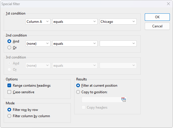
Options of the dialog box
The dialog box for the special filter offers the following options:
▪Range contains headings
| If the first row and/or column of the selected cell range contains headings, enable this option. PlanMaker will then ignore this row or column when filtering. |
▪Case-sensitive
| If this option is enabled, PlanMaker will distinguish between uppercase and lowercase letters in conditions. For a condition such as "COLUMN A equals Smith", the condition will match only if the cell contains the text "Smith". Rows with "SMITH" and "smith" will not be included in the filtering results. |
▪Mode
| This determines whether rows or columns will be filtered. |
| If you select the option Filter row by row, PlanMaker will filter out all rows that do not match the filter condition. |
| If, on the other hand, you select the option Filter column by column, PlanMaker will filter out all columns that do not match the filter condition. |
▪Results
| This determines whether the filter will be applied to the original data or a copy of it: |
| Filter at current position – Select this option and the original data will be filtered. Rows/columns that do not satisfy the filter condition will be hidden at the exact point where you set the filter. |
| Copy to position – If you select this option instead, PlanMaker will create a copy of the original data at a cell address that you specify. This copy contains only the filtered data, and the original data remains unchanged in its place. |
| In the input field under this option, enter where the copy should be inserted. You can either specify a single cell address (which will be the starting point of the output range) or the exact range of cells in which the copy should be placed. Copying to other worksheets is also possible. Caution: If the copy does not fit into this area, it will be truncated accordingly (exception: you specify a single cell address as the starting point). |
Showing all hidden rows again
If you want all rows hidden by the filter to become visible again, choose the ribbon command Data | group Filter | Show all.