Syntax:
FILTER(Range; Include [; IfEmpty])
Description:
This function filters a cell range based on the specified filter conditions and returns it as a list.
Range is the cell range or array from which the values are to be filtered and returned. The range can have one or more columns/rows.
Include is a combination of the two specifications: which column should be searched and which filter criterion this column should contain.
IfEmpty (optional) is the expression you defined if no valid match was found for the Include criterion. The text you enter here will then be returned as the result. If you do not enter anything here and no valid match was found, the function returns the #CALC! error value.
Note:
You can also apply the function to multi-column tables and the output range automatically expands to adjacent cells as needed (simply press the Enter key as usual after entering the formula in the cell). In addition, the result is automatically updated when changes are made to the initial list. For this reason, such formulas are also considered to be functions with a dynamic output range.
If you apply the function to multi-column tables and this causes a spill over to adjacent cells in the results area, a #SPILL! error value will be displayed if those cells are already filled with content. Therefore, make sure that the adjacent area is as empty as needed for the intended expansion of the formula.
Compatibility notes:
Microsoft Excel supports this function only in version 2021 or later. The function is unknown in older versions.
Examples:
Example 1: Filter by one criterion
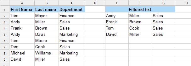
There is a list with multiple names and their department in columns A to C.
The formula FILTER formula is applied in cell E2:
FILTER(A2:C9, C2:C9="Sales") returns a filtered list with the the filter criterion "Sales", which was searched for in column C.
Example 2: Filter by multiple criteria
There is a list with multiple names and their department in columns A to C.
The formula FILTER formula is applied in cell E2:
FILTER(A2:C12, (C2:C12="Sales")*(B2:B12="Miller")) returns a filtered list with the combination of the filter criterion "Sales", which was searched for in column C, and a second criterion "Miller", which was searched for in column B.
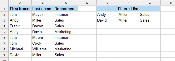
Tip: If you want to combine the filter criteria in such a way that only one of the two criteria has to be fulfilled and not necessarily both, replace the * (AND criterion) with a + (OR criterion).
Example 3: Filter by word components
There is a list with multiple names and their department in columns A to C.
The formula FILTER formula is applied in cell E2:
FILTER(A2:C12, LEFT(B2:B12, 1)="M") returns a filtered list with the filter criterion being the first letter of the value is "M", which was searched for in column B.
Note: The "1" in this formula defines that it is the first character from the beginning of the word. As "1" is the default value (if not specified), it can also be omitted. If, however, you want to specify the first two letters as a filter criterion (e.g. "Mi"), you must enter a "2" here, for example.
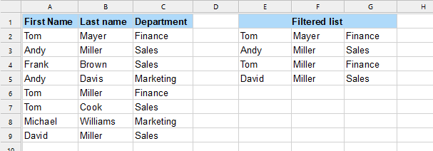
Tip: If you use the term "RIGHT" instead of "LEFT", the program will search for the filter criterion last letter of the value.
Example 4: Apply optional parameter IfEmpty
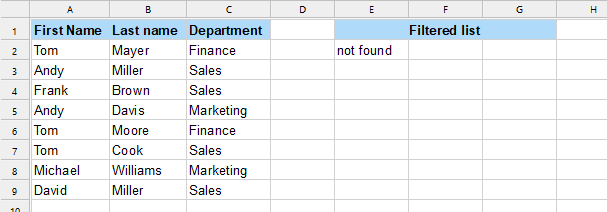
The known list is used again and the FILTER formula is applied in cell E2:
FILTER(A2:C9, C2:C9="Controlling", "not found") returns the expression you defined for the parameter IfEmpty because no match for the filter criterion ("Controlling") was found in column C.
See also: