If the source data is already in the open workbook, proceed as follows:
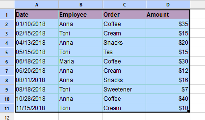
| 1. | Select the entire data area. You can also select just one cell from the source data. PlanMaker will then automatically extend the selection to the entire contiguous area. |
| 2. | Choose the ribbon command Insert | group Tables | Pivot table  . . |
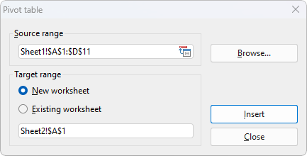
| PlanMaker opens the following dialog box: |
| 3. | Source range: This is the cell range with the existing data from which the pivot table is to be generated. Here, the source range is already defined by your previous selection and can thus be applied. If you still want to change the source range, you can enter the correct cell range in the input field or simply select the correct cell range directly in the worksheet with the mouse. |
Tip: If you have previously given the data area a name (see Naming cell ranges), you can simply enter this name in the input field. An advantage of this procedure is that you only have to adjust the named range if the source data changes.
| 4. | Target range: Here, you can decide where the pivot table should be created. Now choose between the following options: |
| New worksheet: The pivot table will be created in a new worksheet that is automatically generated by PlanMaker. You can adjust the proposed target in the lower input field. |
| Existing worksheet: The pivot table will be created in an existing worksheet. This can be the worksheet containing the source data or another worksheet that has already been created. Please make sure that you first select the option Existing worksheet and only then click on a cell in a free area in the desired worksheet. Alternatively, type the target range into the lower input field. |
Tip: For pivot tables with large amounts of data, we recommend that you use a new worksheet rather than the worksheet with the source data, as it can quickly lead to a lack of space otherwise. If there is only a small amount of data – as in our example – it is useful and illustrative to display the pivot table next to or below the source data in the same worksheet.
| 5. | Confirm with the Insert button to create the pivot table. |
If you created the pivot table in the same worksheet as the source data, the result should look as follows:
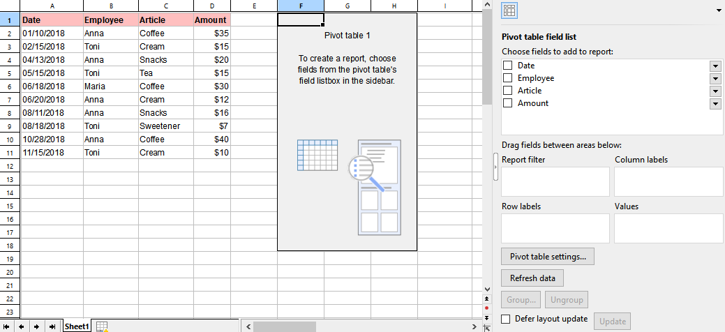
On the left, you can still see the Source data, and the (still blank) Pivot table report next to it. If you click in this report, the Pivot table field list – or just Field list – appears in the right sidebar. It is the central control of the pivot table. By selecting the fields from the field list, you fill the blank pivot table report with content according to your requirements.
For more information about its structure and working with the field list, see Starting with the pivot table field list.