You can use the sort commands on the ribbon tab Data | group Filter to sort a cell range.
Tip: You will also find the commands on the ribbon tab Home| group Contents | Sort and filter.
Simple sorts: Quickly via the direct commands
If you only want to apply the sort to a certain column, you can do this directly via the commands Sort ascending and Sort descending.
You can also select a cell range across multiple columns; in this case, the left column of the selected range is sorted. The selected values to the right of it follow their left value in the same row.
Select the cell range you want to sort, and then on the ribbon tab Data | group Filter, choose one of the following commands:
▪Ascending 
| The data of the selected column is sorted in ascending order (A-Z). |
▪Descending 
| The data of the selected column is sorted in descending order (Z-A). |
If, on the other hand, you want to apply different sort criteria to the columns of a selected cell range or select other user-defined options, choose the command Sort to open the dialog box (see below).
Sort with different criteria: Via the dialog box
You can choose the ribbon command Sort to open a dialog box with additional sort options.
Proceed as follows:
| 1. | Select the cell range to be sorted. |
| 2. | Choose the ribbon command Data| group Filter | Sort  . . |
| 3. | PlanMaker opens the following dialog box: |
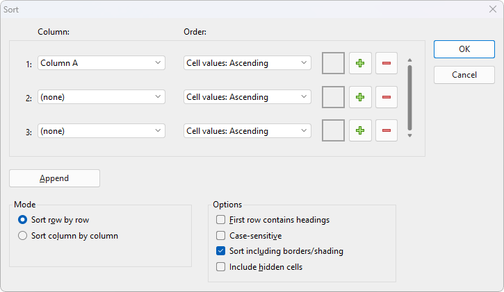
| 4. | For 1:, select the Column by which you want to sort. |
| 5. | To the right of it, you can also change the Order of the sort: You can sort the cell values in Ascending (A to Z) or Descending order (Z to A). |
| Note: If different shades or font colors have been applied to cells, they can also be sorted. See "Sorting cells by shading or font color" below. |
| 6. | If required, you can select additional columns by which to sort for 2: and 3:. |
| If, for example, you select a column containing family names for 1: and a column with first names for 2:, the cell range will be sorted by the family name and then, in groups of identical family names, by the first name. |
| 7. | Make any further settings as required, see below. |
As soon as you confirm with OK, the cell range will be sorted accordingly.
Options of the dialog box
The dialog box offers the following options:
▪Column and Order
| Here, select the desired Column(s) by which to sort. You can also specify the order for each column: Ascending goes from A to Z, and Descending goes from Z to A for the cell values. |
| Note: If different shades or font colors have been applied to cells, they can also be sorted. See "Sorting cells by shading or font color" below. |
| Up to 3 columns can be specified by default. You can even add additional columns if you need more than 3 sort criteria. Up to 64 columns are possible. Proceed as follows: |
| Add a column: Click on the Plus icon to insert another column. |
| Append a column: Click on the Append button (below the list) to append a column at the bottom. |
| Remove a column: Click on the Minus icon to remove the respective column. (This only works if there are more than 3 columns.) |
▪Sort row by row or Sort column by column
| These options determine whether PlanMaker sorts by row or by column. |
▪First row contains headings
| If the first row or column of the selected cell range contains a heading, you should enable this option. PlanMaker then omits it from the sorting. |
| You have selected a list of addresses that you want to sort by row. The first row of your selection contains headings such as "Name", "Street", "City", etc. The actual addresses are in the rows below. You should enable this option so that this row is not sorted and remains the first row. |
▪Case-sensitive
| If you enable this option, sorting distinguishes between uppercase and lowercase letters. For example, all words that begin with a lowercase letter end up in front of the words that begin with a capital letter: |
| Disabled: Apples, bananas, Cherries. Enabled: bananas, Apples, Cherries. |
▪Sort including borders/shading
| If this option is enabled, cells retain their assigned borders and shading when moved by the sorting operation. |
| If disabled, the selected cell range keeps its original formatting as far as borders and shading are concerned. |
▪Include hidden cells
| If the selected range contains cells that have been hidden (see Showing and hiding rows/columns), these are usually not sorted. Enable this option if you want hidden cells to be included in the sort. |
Sorting cells by shading or font color
Not only can you sort a cell range by cell values in ascending/descending order, but you can also sort a range by cell colors (Shades) or text colors (Font colors), provided they have been applied to cells.
Note: The colors do not have their own defined order according to which they can be sorted automatically. Thus, you can decide for yourself which of the available colored cells you would like to move up or down within the cell range.
Proceed as follows:
| 1. | Select the cell range and use the ribbon command Data | group Filter | Sort to open the dialog box as described above. |
| 2. | For 1:, select the Column that you want to sort by color (for example, column A). |
| 3. | Under Order to the right, you can select whether you want to reorder cells according to their cell color or text color, and whether these cells should be sorted to the top or to the bottom. |
| 4. | Then click on the button with the black arrow (to the left of the plus and minus signs) and select the desired color there. Cells of this color are sorted to the very top/to the very bottom. |
| Note: The button with the black arrow appears only if you have specified sorting by cell color/text color in Order. In addition, there must actually be cells in the selected Column that have the relevant colors. |
| 5. | If you specify the same column again for Column 2, Column 3, etc. (for example, column A), you can determine the next color to follow in that column. Make sure that the same sort criterion is set for Order. |
| Otherwise, you can also select other columns for Column 2, Column 3, etc., to which you want to apply further sort criteria. |
As soon as you confirm with OK, the cell range will be sorted accordingly.