The ribbon command Insert | Table ![]() allows you to create "tables" in a worksheet.
allows you to create "tables" in a worksheet.
Note: The fact that this feature is named "table" may be a bit confusing, since the term "table" is often used to represent the content of a worksheet in general. However, since Microsoft has called this feature a "table" in Excel, we decided to keep this term in PlanMaker for compatibility reasons.

How exactly does this feature work?
When you select a cell range and choose the ribbon command Insert | Table, PlanMaker will create a "table" from it.
This has the following effects on the cell range:
▪Automatic formatting with a "table style"
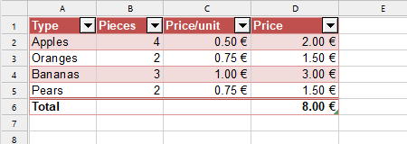
| The selected cell range is formatted automatically with a table style. The default table style alternately applies blue and white shading to the cells. However, you can also use a different style or subsequently change the style and thus change the formatting of the entire "table" at the touch of a button. |
▪AutoFilter applied automatically
| In addition, an AutoFilter is applied to the cell range that was used to create the "table". The AutoFilter adds little arrows to the right of each of the column headings in the table. If you click on one of these arrows, the program will open a menu in which you can set a filter on the cell contents of the corresponding column. |
▪Total row
| In "tables", you can easily activate a total row that is displayed below the table. The total row can display calculations that sum up the values contained in the table (for example, the sum of each column). |
▪Special cell references
| When you have created a "table" in a worksheet, you can also use special cell references. For example, the cell contents in a column of a table can be addressed via its column heading – as in: |
| =SUM(Table3[Spring]) |
The following pages contain everything you need to know about the "table" feature. The following topics are covered:
▪Creating tables in worksheets
▪Removing tables from worksheets
▪Formatting tables in worksheets