Syntax:
XLOOKUP(Crit; SearchRange; ReturnRange [; IfNotFound] [; MatchMode] [; SearchMode])
Description:
This function searches for the first occurrence of the search criterion in the specified SearchRange. If found, the function returns the content of the cell located in the same row in the ReturnRange (for tables that are to be read vertically). For tables that are to be read horizontally, the function returns the content of the cell located in the same column in the ReturnRange. For simplicity purposes, only the vertical search direction is considered in the following explanations.
Note: While VLOOKUP only works in a vertical search direction and HLOOKUP only in a horizontal direction, XLOOKUP can search both vertically and horizontally and also return whole rows/columns as a result.
Important: XLOOKUP uses an exact match by default – unlike VLOOKUP or HLOOKUP, which expect an approximate search without the sort argument.
Crit is the value for which the search is performed. The search is case-insensitive.
SearchRange is the cell range to be evaluated and may only be one column wide. The values can be text strings, numbers or logical values.
ReturnRange is the range with the values to be output. These values are in the same row as the search criterion if the search direction is vertical. The return range can be one or more columns in size.
IfNotFound (optional) is the expression you defined if no valid match was found for the search criterion. The text you enter here will then be returned as the result. If this argument is omitted (default setting) and no valid match is found, the function returns the #NV error value.
MatchMode (optional) controls the type of match. Possible values:
0 = exact match. This is the default value (thus also applies if the argument is omitted). If no exact match is found, the #NV error value is returned or the text defined in the IfNotFound argument.
-1 = If there is no exact match, the next smallest element is returned (ReturnRange must be sorted in descending order).
1 = If there is no exact match, the next largest element is returned (ReturnRange must be sorted in ascending order).
2 = Lets the function know that wildcard characters ("*", "?" and "~") occur in the search criterion.
SearchMode (optional) controls the search direction / search method: Possible values:
1 = Search from top to bottom (in vertical search direction). This is the default value and thus also applies if the argument is omitted.
-1 = Search from bottom to top (in vertical search direction).
2 = Perform a binary search (fast with large data sets) – requires sorted data in ascending order.
-2 = Perform a binary search (fast with large data sets) - requires sorted data in descending order.
Notes:
▪You can also apply the function to multi-column tables and the output range automatically expands to adjacent cells as needed (simply press the Enter key as usual after entering the formula in the cell). In addition, the result is automatically updated when changes are made to the initial list. For this reason, such formulas are also considered to be functions with a dynamic output range.
| If you apply the function to multi-column tables and this causes a spill over to adjacent cells in the results area, a #SPILL! error value will be displayed if those cells are already filled with content. Therefore, make sure that the adjacent area is as empty as needed for the intended expansion of the formula. |
▪XLOOKUP does not require a contiguous cell range of SearchRange and ReturnRange. The ReturnRange can also be to the left of the SearchRange (for tables that are to be read vertically) or even in other worksheets or workbooks.
▪If the dimensions of the SearchRange and ReturnRange do not match (different number of rows for tables that are to be read vertically), the function returns the #VALUE! error value.
▪If no match is found and the IfNotFound argument is not specified, the function returns the #NV error value.
▪Wildcards (*, ?, ~) can be used when matching with MatchMode = 2.
▪XLOOKUP is not case-sensitive by default. The only way to achieve real case sensitivity is to use additional functions/combinations (e.g., formula EXACT ).
▪For approximate matches (MatchMode = 1 or -1 or binary search modes), the data in the SearchRange must be sorted in the required order – otherwise the results will not be reliable.
Compatibility notes:
Microsoft Excel supports this function only in version 2021 or later. The function is unknown in older versions.
Examples (vertical search direction):
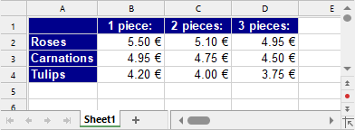
You sell flowers at different unit prices depending on the amount of flowers the customer buys. To do so, you have created a table with a discount scale:
You can now use the XLOOKUP function to determine the price for a specific type of flower depending on the number of pieces.
Use the following arguments:
For Crit, you enter the name of the flower type (i.e., "roses", "carnations" or "tulips").
For SearchRange, you enter the cell range containing the flower types – in this case, the first column with the range A2:A4.
For ReturnRange, you enter the cell range containing the prices. The price for 1 piece is in column 2 of the selected range, the price for 2 pieces in column 3 and the price for 3 pieces in column 4. You can now either specify a range consisting of one column (e.g., B2:B4) or several columns (e.g., B2:D4).
You can optionally use the IfNotFound argument for cases in which no valid match was found. Instead of the #NV error value, an expression defined by you (e.g., "not available") is returned.
Examples (vertical search direction):
XLOOKUP("Roses", A2:A4, B2:B4) returns the unit price when purchasing 1 rose, i.e., 5.50.
XLOOKUP("Roses", A2:A4, C2:C4) returns the unit price when purchasing 2 roses, i.e., 5.10.
XLOOKUP("Roses", A2:A4, D2:D4) returns the unit price when purchasing 3 roses, i.e., 4.95.
XLOOKUP("Carnations", A2:A4, D2:D4) returns 4.50.
XLOOKUP("Petunias", A2:A4, D2:D4) returns the #N/A error value because "Petunias" does not appear in A2:A4.
XLOOKUP("Petunias"; A2:A4; D2:D4; "not available"), however, returns the "not available" text you defined for the IfNotFound argument.
XLOOKUP("Roses"; A2:A4; B2:D4) returns all unit prices when purchasing 1, 2 or 3 roses next to each other in one row.
Example (horizontal search direction):

XLOOKUP("Roses";B1:D1;B2:D2) returns the unit price when purchasing 1 rose, i.e., 5.50.
Example (approximate search):
The following example explains the use of the MatchMode argument.
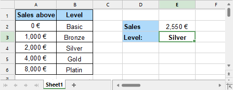
As a customer, you reach a higher bonus level depending on the sales volume achieved. You have created a table in vertical search direction with the following bonus levels:
Note: The IfNotFound argument should be omitted for this table (default setting). However, it must be entered in the formula with the character string ,, as the 4th argument so that the 5th argument, MatchMode, appears in the correct position for the formula to work.
XLOOKUP(E2, A2:A6, B2:B6, , -1) returns the bonus level "Silver", as the exact matching value for a sales volume of 2,550 cannot be found and the next smallest element (in the SearchRange: 2000) is returned (in the ReturnRange: Silver).
Tip: For the search criterion, there are generally the alternative options of specifying it as an expression (e.g., "Roses" as in the examples above) or as a cell containing the value you are looking for (as here, for example, with cell "E2").
See also: