FreeOffice: The Data consolidation feature is not included in SoftMaker FreeOffice.
As mentioned in the introduction of the section Consolidating data, the command Data consolidation allows you to consolidate data from one or more cell ranges, for example, in order to calculate their total sums.
In addition to consolidating data by its position (see previous section), data can also be consolidated by its labels. This works as follows:
The data to be evaluated can be stored in any number of "source ranges" – all of which should have one thing in common: a label has been added to each value (for example, in the cell to the left of the value).
When you start a consolidation with such source ranges and enable the option Labels in left column, PlanMaker calculates the sum of all values that have the same label on their left.
The same label may occur as often as desired. The size of the individual source ranges and the order of the data within them are irrelevant. PlanMaker only uses the labels to determine which data is to be consolidated.
Example
A fruit shop offers different types of fruit. Each individual sale during the course of a day is recorded in a worksheet. You now want to calculate how much of each type of fruit was sold in total.
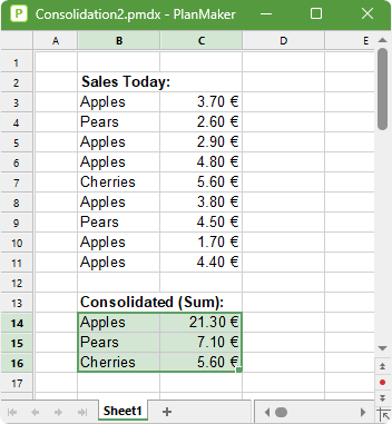
Of course, the individual types of fruit occur in a completely random order, but this is irrelevant to the consolidate command:
Simply choose the command Data consolidation. Add the cell range with the individual sales as the source range (B3:C11 in this case). Note: This must contain the numbers and their labels! Then select any target range for the result (B14:C16 in the figure) and confirm.
Result: The totals of the sales of the individual types of fruit appear in the target range.
Performing a consolidation by labels
To consolidate data by its labels, proceed as follows:
| 1. | Enter the data to be consolidated into one or more cell ranges. The size and structure of these cell ranges don't matter. However, the values to be consolidated should all have a label – either in the column to the left of them and/or in the row above them. |
| The individual cell ranges can all be in the same worksheet, in multiple worksheets or even in several different documents. |
| 2. | Choose the ribbon command Data | group Analyze | Data consolidation |
| 3. | Click into the Source ranges input field. There, enter the address of the cell range with the data to be consolidated. See also notes at the end of the previous section. |
| Tip: Alternatively, you can also click directly into the worksheet while the dialog box is open and simply select the cell range in the worksheet with the mouse to transfer it to the dialog box. |
Important: Each source range must contain both the values themselves and their labels. The labels must be in the far left column or in the top row of the range.
| 4. | Click on the Add button. |
| 5. | To add additional source ranges, repeat steps 3. and 4. |
| 6. | For Target range, enter the address of the cell range in which you want the result of the consolidation to be inserted. |
| Tip: It is sufficient to specify the address of the cell in the top left corner of the target range. PlanMaker will then determine its size automatically. |
| Tip: You can also simply click on the desired cell directly in the worksheet to transfer its address to the dialog box. |
| 7. | For Function, select the arithmetic function to be used for the consolidation. |
| 8. | For Options, specify the position of the labels in the source ranges: |
| Labels in left column: The labels are stored in the far left column of each source range. (The associated data must then be entered directly to the right of it.) |
| Labels in top row: The labels are stored in the top row of each source range. (The associated data must then be entered directly below.) |
| You can also enable both options if you want to evaluate source ranges where labels are in their far left column and in their top row. |
| If you enable the option Sort labels, the results of the consolidation in the target range will be sorted according to the labels. |
| 9. | Click on Apply to start the consolidation. |
The data from the source ranges is now consolidated using the selected arithmetic function, and the result is inserted in the target range.
Note: The result of a consolidation is inserted into the worksheet as fixed numbers. These numbers will not be updated if you change the values in any of the source ranges.
This command is thus primarily useful if you want to evaluate the current state of data and no longer want to take changes into account (useful, for example, for monthly reports). For more information, see also Editing and updating consolidations.